Requirements

zREngine requires:

• a version of APL+Win at least equal to v17+⁽¹⁾
• the .Net Framework v4.7+
• that R 32-bits be installed on your computer (R 64-bits may also be installed but is not used by zREngine)⁽²⁾

⁽¹⁾ zREngine also works with APL+Win v16.x but does not support high DPI screens as well as with APL+Win v17+
⁽²⁾ The zzrengine demo APL function in the distributed zREngine.w3 workspace contains instructions about the proper zREngine installation and about where to download the R v3.3+ language from.

Download

Download the zREngine product:

Download »

Demos

The zREngine.w3 workspace includes 2 demos showing you how to use R from APL+Win: once you have properly installed zREngine, just load the zREngine.w3 workspace and run:

      ]demo zzrengine

or run:

      ]demo zzrengine2

The zzrengine2 demo demonstrates how to use the ggplot2 graphics package from APL+Win.

Note: to run the above demos you must have the APL+Win User Command Processor up and running and must have the following file in your User Commands file list: UCMDS3 (as found in your APL+Win v17+ folder).

Description

With zREngine you can:

• use any R command from APL+Win using the Eval method
• display any R statistical plot in an APL+Win form using the EvalPlot or EvalGGPlot methods
• return results to APL from R statistical procedures
• display the R Console in an APL+Win Form and use it
• use some zREngine utilities to more easily pass arguments to the Eval method

Using zREngine in your own APL application

To use zREngine in your own application, you simply need to copy (or pcopy) the entire zRengine.w3 workspace into your own workspace

There should normally not be any name conflicts as all zREngine functions start by a z followed by an uppercase letter (or a z followed by only lowercase letters)

Examples

You must first run the zzInit utility to setup the zObjects system and register the zREngine custom APL object

      zzInit

Note: the zzInit function is automatically run when you load the zREngine workspace.

You must then create an instance of the zREngine custom APL object:

      ←'zr'⎕wi'*Create' 'zREngine'

Note: the zzre utility is a handy easy to type function for running zzInit and creating an instance of zREngine.

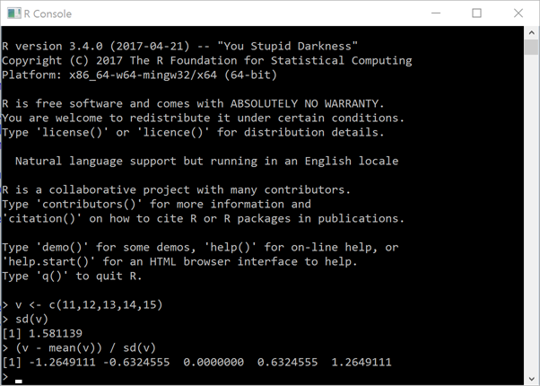
The first thing you can do is to display the R-Console in an APL+Win Form in your application and let the user use R to compute some statistics. In the following example, we create an R vector v and compute its Standard Deviation and then its z-score:

      ←'zr'⎕wi'RConsole'

The rpath property returns the path of the R executable:

      'zr'⎕wi'rpath'
C:\Program Files\R\R-3.4.2\bin\i386

Let's use the Eval method to create an R variable and then query its value

      'zr'⎕wi'Eval' 'aaa = 123'
      'zr'⎕wi'Eval' 'aaa'
123

You can use the EvalPlot method to display an R plot in an APL+Win Form as follows:

      'zr'⎕wi'EvalPlot' 'ff' 'plot(cars)'7 1

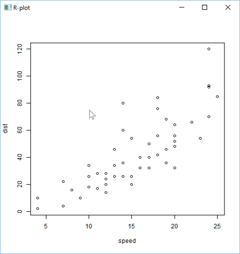
You just need to indicate the name of the APL+Win Form object you want to create (here: 'ff') and the R instruction to run to create the plot (here: 'plot(cars)'). Note that we have not defined the cars R variable, but it works because cars is one of the many sample data sets delivered with R.

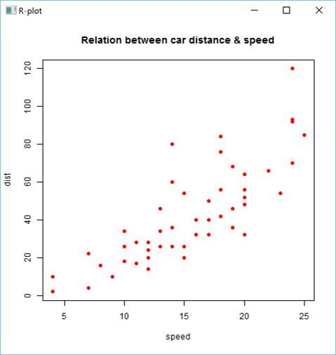
You can improve R plots by adding titles, using colors, etc.. Example:

      'zr'⎕wi'EvalPlot' 'ff' 'plot(cars, main="Relation between car distance & speed", pch=19, col="red")'7 1

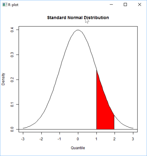
Here is a more sophisticated example:

      'zr'⎕wi'Eval' 'x <- seq(from=-3, to=+3, length.out=100)'
      'zr'⎕wi'Eval' 'y <- dnorm(x)'

      s←''
      s,←⊂'plot(x, y, main="Standard Normal Distribution", type="l", ylab="Density", xlab="Quantile")'
      s,←⊂'abline(h=0)'
      s,←⊂'region.x <- x[1 <=x & x<=2]'
      s,←⊂'region.y <- y[1 <=x & x<=2]'
      s,←⊂'region.x <- c(region.x[1], region.x, tail(region.x,1))'
      s,←⊂'region.y <- c(          0, region.y,                0)'
      s,←⊂'polygon(region.x, region.y, density=-1, col="red")'

      'zr'⎕wi'EvalPlot' 'ff's 8 1

You can create R Data Frames from APL+Win nested arrays easily:

      s←0 4⍴''
      s⍪←'City'    'ProductA' 'ProductB' 'ProductC'
      s⍪←'Seattle'        23         11         12
      s⍪←'London'         89          6         56
      s⍪←'Tokyo'          24          7         13
      s⍪←'Berlin'         36         34         44
      s⍪←'Mumbai'          3         78         14
      'zr'⎕wi'CreateDataFrame' 'sales' s

At any time you can use the verbose property to display in the APL Session the R commands that are run by zREngine when you run some commands:

      'zr'⎕wi'verbose'1

      s←0 4⍴''
      s⍪←'City'    'ProductA' 'ProductB' 'ProductC'
      s⍪←'Seattle'        23         11         12
      s⍪←'London'         89          6         56
      s⍪←'Tokyo'          24          7         13
      s⍪←'Berlin'         36         34         44
      s⍪←'Mumbai'          3         78         14
      'zr'⎕wi'CreateDataFrame' 'sales' s
rEng.Evaluate(@"col1<-c(""Seattle"",""London"",""Tokyo"",""Berlin"",""Mumbai"")");
rEng.Evaluate(@"col2<-c(23,89,24,36,3)");
rEng.Evaluate(@"col3<-c(11,6,7,34,78)");
rEng.Evaluate(@"col4<-c(12,56,13,44,14)");
rEng.Evaluate("sales = as.data.frame(list(City=col1,ProductA=col2,ProductB=col3,ProductC=col4))");

The last 5 lines displayed in the APL Session are the R commands that have been run when you used the CreateDataFrame method.

Once you have the Data Frame defined in R, you can plot it in various manners:

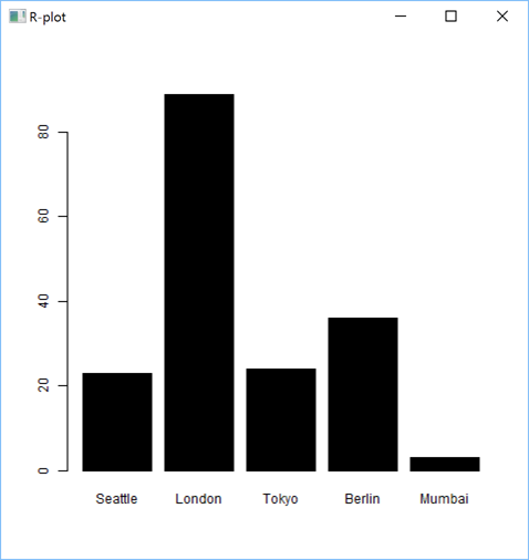
      'zr'⎕wi'EvalPlot' 'ff' 'barplot(sales$ProductA, names.arg=sales$City, col="black")' 8 1

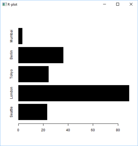
      'zr'⎕wi'EvalPlot' 'ff' 'barplot(sales$ProductA, names.arg=sales$City, horiz=TRUE, col="black")' 8 1

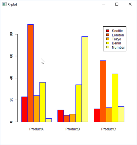
      'zr'⎕wi'EvalPlot' 'ff' 'barplot(as.matrix(sales[,2:4]), beside=TRUE, legend=sales$City, col=heat.colors(5), border="blue")' 8 1

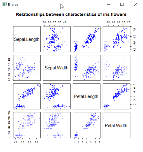
You can create plots which would be difficult to create in APL, like Pair Plots:

      'zr'⎕wi'EvalPlot' 'ff' 'plot(iris[,1:4], main="Relationships between characteristics of iris flowers", pch=19, col="blue", cex=0.9)' 8 1

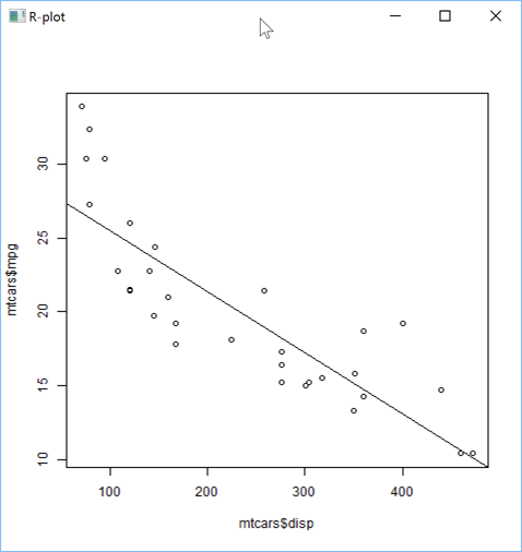
Here is how you can create a linear regression plot:

      'zr'⎕wi'Eval' 'x <- (1:100)/10'
      'zr'⎕wi'Eval' 'y <- 100+10*exp(x/2) + rnorm(x)/10'
      s←''
      s,←⊂'plot(mtcars$mpg~mtcars$disp)'
      s,←⊂'lmfit<-lm(mtcars$mpg~mtcars$disp)'
      s,←⊂'abline(lmfit)'
      'zr'⎕wi'EvalPlot' 'ff' s 8 1

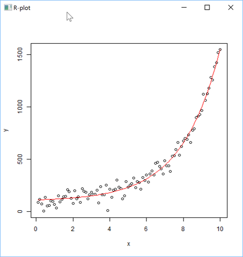
or a non linear regression plot:

      'zr'⎕wi'Eval' 'x <- (1:100)/10'
      'zr'⎕wi'Eval' 'y <- 100+10*exp(x/2) + rnorm(x)*50'
      'zr'⎕wi'Eval' 'nlmod<-nls(y~Const+A*exp(B*x), trace=TRUE)'
      s←''
      s,←⊂'plot(x,y)'
      s,←⊂'lines(x, predict(nlmod), col="red")'
      'zr'⎕wi'EvalPlot' 'ff' s 8 1

You can then easily retrieve the values predicted by the model:

      'zr'⎕wi'Eval' 'predict(nlmod)'
111.2006823 111.8198837 112.4694778 113.1509563 113.8658844 114.6159038 115.4027369 116.2281907 117.0941608 118.0026359 118.9557023 119.9555488
      121.0044714 122.104879 123.2592987 124.4703816 125.7409089 127.0737984 128.472111 129.939058 131.4780082 133.0924957 134.7862283 136.5630955
      138.4271779 140.3827564 142.4343219 144.5865858 146.8444908 149.2132221 151.6982195 154.3051898 157.0401198 159.9092903 162.9192903 166.0770322
      169.3897677 172.8651046 176.5110239 180.3358983 184.3485117 188.5580791 192.9742676 197.6072189 202.4675726 207.5664904 212.915682 218.5274317
      224.4146268 230.5907872 237.0700964 243.8674341 250.9984102 258.479401 266.3275865 274.5609899 283.1985193 292.2600105 301.7662732 311.7391384
      322.2015088 333.1774109 344.6920509 356.771872 369.4446155 382.739384 396.6867089 411.3186201 426.6687196 442.7722587 459.6662191 477.3893975
      495.982495 515.4882106 535.9513387 557.4188729 579.940113 603.5667788 628.3531288 654.3560845 681.6353614 710.253606 740.27654 771.7731105
      804.8156492 839.4800379 875.8458829 913.9966981 954.0200963 996.0079909 1040.056807 1086.267701 1134.746797 1185.605427 1238.960385 1294.934203
      1353.655423 1415.258897 1479.886097 1547.685439

or retrieve the regression coefficients:

      'zr'⎕wi'Eval' 'coef(nlmod)[1]'         ⍝ Const
98.58546722
      'zr'⎕wi'Eval' 'coef(nlmod)[2]'         ⍝ A
12.02498437
      'zr'⎕wi'Eval' 'coef(nlmod)[3]'         ⍝ B
0.4791711418

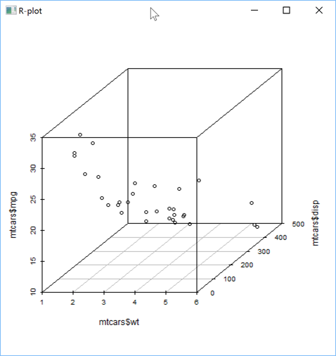
You can also create 3D plots, like a 3D scatter plot, but for that you need to install an R package.

This can be easily done using the R install.packages command: here we'll install the scatterplot3d package.

      'zr'⎕wi'Eval' 'if(!require("scatterplot3d")) {install.packages("scatterplot3d")}'

      'zr'⎕wi'Eval' 'library(scatterplot3d)'
 scatterplot3d maps stats graphics grDevices utils datasets methods base

You can then display the 3D scatter plot:

      'zr'⎕wi'EvalPlot' 'ff' 'scatterplot3d(x=mtcars$wt, y=mtcars$disp, z=mtcars$mpg)' 8 1

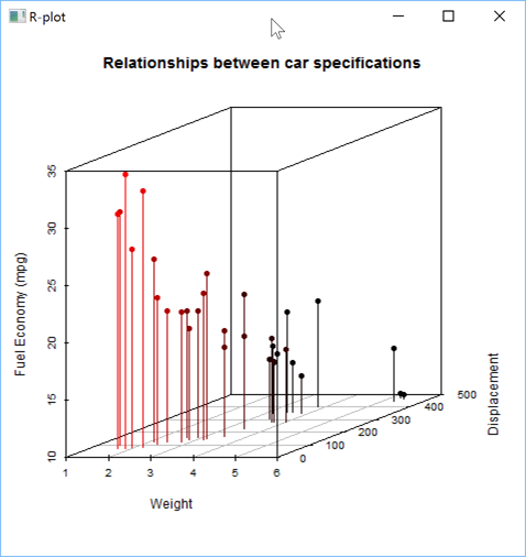
or with some additional parameters to customize the chart:

      s←''
      s,←'scatterplot3d(x=mtcars$wt, y=mtcars$disp, z=mtcars$mpg,'
      s,←'pch=16, highlight.3d=TRUE, angle=20,'
      s,←'xlab="Weight", ylab="Displacement", zlab="Fuel Economy (mpg)",'
      s,←'type="h",'
      s,←'main="Relationships between car specifications")'

      'zr'⎕wi'EvalPlot' 'ff' s 8 1

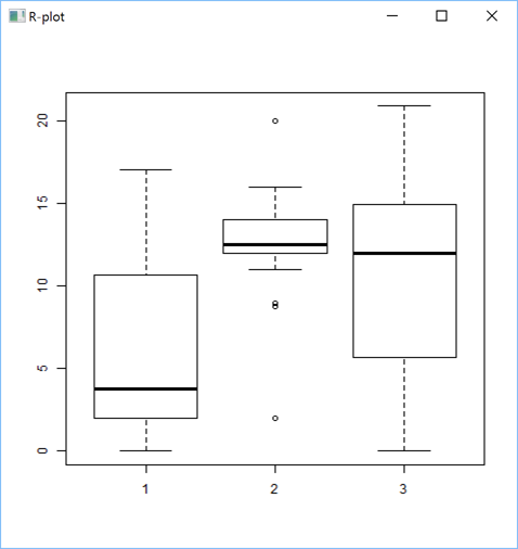
Let's now create a Box Plot using the USCereal variable from the MASS package:

      'zr'⎕wi'Eval' 'data(UScereal, package="MASS")'
 UScereal

      'zr'⎕wi'EvalPlot' 'ff' 'boxplot(sugars~shelf, data=UScereal)' 8 1

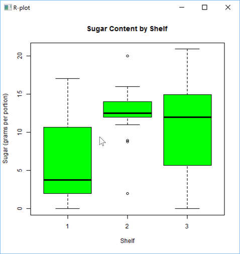
or with some adornments:

      'zr'⎕wi'EvalPlot' 'ff' 'boxplot(sugars~shelf, data=UScereal, main="Sugar Content by Shelf", xlab="Shelf", ylab="Sugar (grams per portion)", col="green")' 8 1

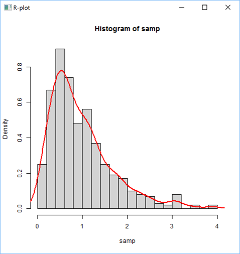
Now drawing a Density Estimate over a Histogram:

      s←''
      s,←⊂'samp <- rgamma(500,2,2)'
      s,←⊂'hist(samp, 20, prob=T, col="lightgray")'
      s,←⊂'lines(density(samp), col="red", lwd=2)'

      'zr'⎕wi'EvalPlot' 'ff' s 8 1

zREngine is not just useful for drawin statistical plots, but can be used to do any statistical calculations. The results can then be retrieved in APL. Here is an example:

Let's start by doing a simple regression:

      'zr'⎕wi'Eval' 'x<-1:100'
      'zr'⎕wi'Eval' 'y<-(x*2)+rnorm(x)/10'
      'zr'⎕wi'Eval' 'model <- lm(y~x)'

We can now query the resulting model objet for various statistical results:

      ⍝ 1. the ANOVA table

      'zr'⎕wi'Eval' 'anova(model)'
 Df           Sum Sq            Mean Sq          F value           Pr(>F)
  1 333288.782800000 333288.78280000000  3.243061075E7    2.74430227E¯272
 98      1.007144175      0.01027698138  ?.?<0000000E316  ?.?<000000E317

      ⍝ 2. the regression coefficients

      'zr'⎕wi'Eval' 'coef(model)'
0.006421721218 1.999966345

      ⍝ 3. the confidence intervals for the regresison coefficients

      'zr'⎕wi'Eval' 'confint(model)'
¯0.03411720069 1.999269415 0.04696064313 2.000663275

      ⍝ 4. the residual sum of squares

      'zr'⎕wi'Eval' 'deviance(model)'
1.007144175

      ⍝ 5. the vector of orthogonal effects

      'zr'⎕wi'Eval' 'effects(model)'
¯1010.047221 577.311686 ¯0.06944103833 0.003236398264 0.1110455067 0.04254541479 ¯0.1043375201 0.08335218672 ¯0.03221809368 0.1170143052 0.01592253738
      0.176713285 ¯0.01938207056 ¯0.1581178283 ¯0.07932506707 0.03095129846 0.1697287573 ¯0.1659089279 ¯0.1027564124 0.1555413197 0.3005808348
      0.133270387 0.01828492149 0.1264371516 ¯0.1764631639 0.06989438887 0.042160908 0.006834558259 0.04121117656 ¯0.0813920313 ¯0.09656304067
      0.0008283179866 ¯0.240766567 0.02037260115 ¯0.05503776352 ¯0.09973439873 0.0001869506567 0.01880467442 ¯0.02315901968 ¯0.1407270808 ¯0.1243225415
      0.2050677578 ¯0.1714243548 ¯0.003198118028 0.04497587026 ¯0.2381329266 0.08818532755 0.04357344597 ¯0.004060070658 ¯0.1034713937 ¯0.02000421575
      0.05491019043 0.1203195819 0.001587561635 0.1065930323 0.1432600441 ¯0.04782385586 0.09995279881 ¯0.06547390911 ¯0.02378485653 ¯0.09600055829
      0.1557762956 0.01322598882 ¯0.008363468836 ¯0.02956315859 0.06880327537 0.06796314267 ¯0.1403239099 ¯0.01010772678 ¯0.09148278906 0.03462108024
      0.01874689764 0.04392282327 0.1739325261 ¯0.0008175915554 0.03280409869 0.02998408256 0.02101436161 ¯0.05443950747 0.09468324007 0.08361540744
      ¯0.1083622026 ¯0.01392251456 ¯0.0833796958 0.05913886961 0.02638602687 0.04728581716 0.0815456235 ¯0.08276132467 0.08593170512 0.2865907257
      0.01408885434 0.0775280696 0.1556698974 ¯0.01224490722 0.05873519554 ¯0.0001580060435 ¯0.02739532405 0.05838645028 0.04200392781

      ⍝ 6. the vector of fitted y values

      'zr'⎕wi'Eval' 'fitted(model)'
2.006388066 4.006354411 6.006320756 8.006287101 10.00625345 12.00621979 14.00618614 16.00615248 18.00611882 20.00608517 22.00605151 24.00601786
      26.0059842 28.00595055 30.00591689 32.00588324 34.00584958 36.00581593 38.00578227 40.00574862 42.00571496 44.00568131 46.00564765 48.005614
      50.00558034 52.00554669 54.00551303 56.00547938 58.00544572 60.00541207 62.00537841 64.00534476 66.0053111 68.00527745 70.00524379 72.00521014
      74.00517648 76.00514283 78.00510917 80.00507552 82.00504186 84.00500821 86.00497455 88.00494089 90.00490724 92.00487358 94.00483993 96.00480627
      98.00477262 100.004739 102.0047053 104.0046717 106.004638 108.0046043 110.0045707 112.004537 114.0045034 116.0044697 118.0044361 120.0044024
      122.0043688 124.0043351 126.0043014 128.0042678 130.0042341 132.0042005 134.0041668 136.0041332 138.0040995 140.0040659 142.0040322 144.0039986
      146.0039649 148.0039312 150.0038976 152.0038639 154.0038303 156.0037966 158.003763 160.0037293 162.0036957 164.003662 166.0036283 168.0035947
      170.003561 172.0035274 174.0034937 176.0034601 178.0034264 180.0033928 182.0033591 184.0033254 186.0032918 188.0032581 190.0032245 192.0031908
      194.0031572 196.0031235 198.0030899 200.0030562

      ⍝ 7. the model residuals

      'zr'⎕wi'Eval' 'resid(model)'
¯0.1142236174 0.1139857538 ¯0.06374886979 0.008554703229 0.1159899481 0.0471159926 ¯0.1001408059 0.08717503738 ¯0.02876910659 0.1200894287 0.01862379732
      0.1790406814 ¯0.01742853778 ¯0.1565381591 ¯0.07811926144 0.03178324052 0.1701868358 ¯0.165824713 ¯0.1030460611 0.1548778075 0.2995434589
      0.1318591476 0.01649981852 0.1242781851 ¯0.178995994 0.06698769516 0.03888035072 0.003180137405 0.03718289213 ¯0.08579417931 ¯0.1013390523
      ¯0.004321557171 ¯0.2462903058 0.01447499884 ¯0.06130922941 ¯0.1063797282 ¯0.00683224238 0.01141161781 ¯0.03092593987 ¯0.1488678646 ¯0.1328371888
      0.1961792469 ¯0.1806867293 ¯0.01283435609 0.03496576861 ¯0.2485168918 0.07742749875 0.0324417536 ¯0.0155656266 ¯0.1153508132 ¯0.03225749885
      0.04228304376 0.1073185717 ¯0.01178731219 0.09284429489 0.1291374432 ¯0.06232032041 0.08508247068 ¯0.08071810081 ¯0.03940291181 ¯0.1119924771
      0.1394105131 ¯0.003513657185 ¯0.02547697842 ¯0.04705053175 0.05094203864 0.04972804236 ¯0.1589328737 ¯0.02909055424 ¯0.1108394801 0.01489052562
      ¯0.001357520552 0.02344454151 0.1530803807 ¯0.02204360047 0.0112042262 0.008010346493 ¯0.001333238037 ¯0.07716097069 0.07158791327 0.06014621707
      ¯0.1322052565 ¯0.03813943208 ¯0.1079704769 0.03417422494 0.00104751862 0.02157344533 0.05545938809 ¯0.1092214236 0.05909774256 0.2593828996
      ¯0.01349283536 0.04957251632 0.1273404806 ¯0.04094818765 0.02965805153 ¯0.02960901363 ¯0.05722019521 0.02818771555 0.0114313295

      ⍝ 8. the variance-covariance matrix of the main parameters

      'zr'⎕wi'Eval' 'vcov(model)'
0.0004173077288 ¯0.000006228473565 ¯0.000006228473565 1.233361102E¯7

It is also possible to retrieve a summary of the model by using the R summary() R function:

            ⊃'zr'⎕wi'Eval' 'summary(model)'

Call:
lm(formula = y ~ x)

Residuals:
      Min        1Q    Median        3Q       Max
-0.248517 -0.062677  0.002114  0.052071  0.299543

Coefficients:
             Estimate Std. Error  t value Pr(>|t|)
(Intercept) 0.0064217  0.0204281    0.314    0.754
x           1.9999663  0.0003512 5694.788   <2e-16 ***
---
Signif. codes:  0 '***' 0.001 '**' 0.01 '*' 0.05 '.' 0.1 ' ' 1

Residual standard error: 0.1014 on 98 degrees of freedom
Multiple R-squared:      1,	Adjusted R-squared:      1
F-statistic: 3.243e+07 on 1 and 98 DF,  p-value: < 2.2e-16

or even get more details using the R str() function:

      ⊃'zr'⎕wi'Eval' 'str(model)'
List of 12
 $ coefficients : Named num [1:2] 0.00642 1.99997
  ..- attr(*, "names")= chr [1:2] "(Intercept)" "x"
 $ residuals    : Named num [1:100] -0.11422 0.11399 -0.06375 0.00855 0.11599 ...
  ..- attr(*, "names")= chr [1:100] "1" "2" "3" "4" ...
 $ effects      : Named num [1:100] -1.01e+03 5.77e+02 -6.94e-02 3.24e-03 1.11e-01 ...
  ..- attr(*, "names")= chr [1:100] "(Intercept)" "x" "" "" ...
 $ rank         : int 2
 $ fitted.values: Named num [1:100] 2.01 4.01 6.01 8.01 10.01 ...
  ..- attr(*, "names")= chr [1:100] "1" "2" "3" "4" ...
 $ assign       : int [1:2] 0 1
 $ qr           :List of 5
  ..$ qr   : num [1:100, 1:2] -10 0.1 0.1 0.1 0.1 0.1 0.1 0.1 0.1 0.1 ...
  .. ..- attr(*, "dimnames")=List of 2
  .. .. ..$ : chr [1:100] "1" "2" "3" "4" ...
  .. .. ..$ : chr [1:2] "(Intercept)" "x"
  .. ..- attr(*, "assign")= int [1:2] 0 1
  ..$ qraux: num [1:2] 1.1 1.15
  ..$ pivot: int [1:2] 1 2
  ..$ tol  : num 1e-07
  ..$ rank : int 2
  ..- attr(*, "class")= chr "qr"
 $ df.residual  : int 98
 $ xlevels      : Named list()
 $ call         : language lm(formula = y ~ x)
 $ terms        :Classes 'terms', 'formula'  language y ~ x
  .. ..- attr(*, "variables")= language list(y, x)
  .. ..- attr(*, "factors")= int [1:2, 1] 0 1
  .. .. ..- attr(*, "dimnames")=List of 2
  .. .. .. ..$ : chr [1:2] "y" "x"
  .. .. .. ..$ : chr "x"
  .. ..- attr(*, "term.labels")= chr "x"
  .. ..- attr(*, "order")= int 1
  .. ..- attr(*, "intercept")= int 1
  .. ..- attr(*, "response")= int 1
  .. ..- attr(*, ".Environment")=<environment: R_GlobalEnv>
  .. ..- attr(*, "predvars")= language list(y, x)
  .. ..- attr(*, "dataClasses")= Named chr [1:2] "numeric" "numeric"
  .. .. ..- attr(*, "names")= chr [1:2] "y" "x"
 $ model        :'data.frame':	100 obs. of  2 variables:
  ..$ y: num [1:100] 1.89 4.12 5.94 8.01 10.12 ...
  ..$ x: int [1:100] 1 2 3 4 5 6 7 8 9 10 ...
  ..- attr(*, "terms")=Classes 'terms', 'formula'  language y ~ x
  .. .. ..- attr(*, "variables")= language list(y, x)
  .. .. ..- attr(*, "factors")= int [1:2, 1] 0 1
  .. .. .. ..- attr(*, "dimnames")=List of 2
  .. .. .. .. ..$ : chr [1:2] "y" "x"
  .. .. .. .. ..$ : chr "x"
  .. .. ..- attr(*, "term.labels")= chr "x"
  .. .. ..- attr(*, "order")= int 1
  .. .. ..- attr(*, "intercept")= int 1
  .. .. ..- attr(*, "response")= int 1
  .. .. ..- attr(*, ".Environment")=<environment: R_GlobalEnv>
  .. .. ..- attr(*, "predvars")= language list(y, x)
  .. .. ..- attr(*, "dataClasses")= Named chr [1:2] "numeric" "numeric"
  .. .. .. ..- attr(*, "names")= chr [1:2] "y" "x"
 - attr(*, "class")= chr "lm"

ggplot2 Support

You can now fully use the ggplot2 package in zREngine v2

First ensure that the ggplot2 package has been downloaded and is loaded:

      'zr'⎕wi'Eval' 'if(!require("ggplot2")) {install.packages("ggplot2")}'
      'zr'⎕wi'Eval' 'library(ggplot2)'

Here are some examples:

      plot←'ggplot(faithful, aes(x=waiting))'
      plot,←' + geom_line(stat="density", adjust=.25, colour="red")'
      plot,←' + geom_line(stat="density")'
      plot,←' + geom_line(stat="density", adjust=2, colour="blue")'
      ←'zr'⎕wi'EvalGGPlot' 'ff,ggplot2 example' plot fontfactor 1

      plot←'ggplot(faithful, aes(x=waiting, y=..density..))'
      plot,←' + geom_histogram(fill="cornsilk", colour="grey60", size=.2)'
      plot,←' + geom_density()'
      plot,←' + xlim(35,105)'
      ←'zr'⎕wi'EvalGGPlot' 'ff,ggplot2 example' plot fontfactor 1

      plot←'ggplot(faithful, aes(x=eruptions, y=waiting))'
      plot,←' + geom_point()'
      plot,←' + stat_density2d()'
      ←'zr'⎕wi'EvalGGPlot' 'ff,ggplot2 example' plot fontfactor 1

      plot←'ggplot(faithful, aes(x=eruptions, y=waiting))'
      plot,←' + stat_density2d(aes(fill=..density..), geom="raster", contour=FALSE, h=c(.5,5))'
      ←'zr'⎕wi'EvalGGPlot' 'ff,ggplot2 example' plot fontfactor 1